A1. Part 2. External sort. In- and out-degree distribution

1. Introduction

In this part, we start exploring properties of a large Twitter graph, using external-memory algorithms, namely sorting large files using a small constant amount of main memory.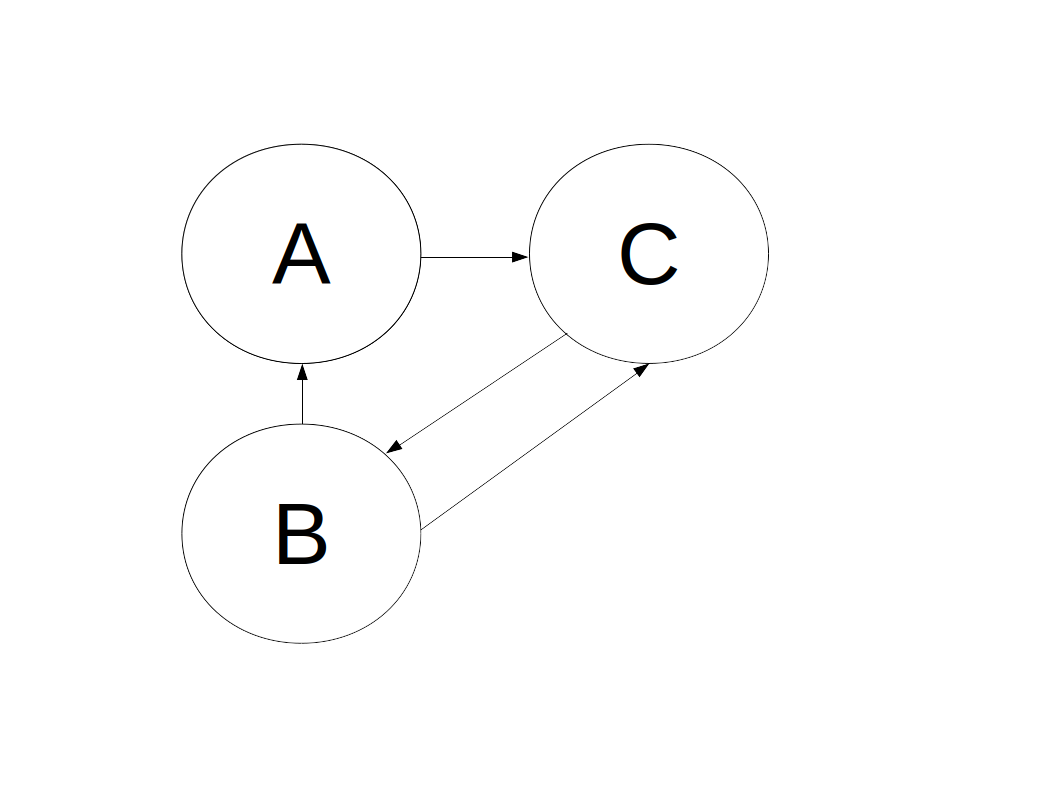

Figure 1. Graph example

 As before, we model the social network in edges.csv as a directed graph. In this graph, if user A followers user C, then there is an outgoing edge from vertex A to vertex C. An out-degree of a vertex is the total number of edges coming out of it. The out-degrees of vertices A, B, and C in Figure 1 are d-out(A) = 1, d-out (B) = 2, and d-out (C)=1. An in-degree of a vertex is the total number of edges coming into it. The in-degrees for A, B and C are 1, 1, and 2 respectively.

One of the most general characteristics of any graph is the distribution of in- and out-degrees. In order to learn about these distributions, we need to count - for each possible degree - the total number of vertices with this degree. Using example in Figure 1, we want to compute histograms of in-degrees and out-degrees, which in this case are the following sequences of (degree,count) pairs: (1,2), (2,1) for out-degrees, and (1,2), (2,1) for in-degrees.

Our main research goal is to find, for each value of k, how many users have k inbound-links (the measure of popularity), and how many users have k outbound-links (the measure of conformism). Often, social network datasets exhibit a power-low distribution. That means that for each value of k, there are 1/k^c vertices with this number of in- or out-links. First, we will test if the distributions for this dataset follow the power law, and if they do, we will determine the power of each distribution - the c parameter in each formula.

While computing the out-degree of each vertex in the dataset sorted by UID1 is trivial (and can be done with a slight modification of your max-average program for A 1.1.), finding the number of in-degrees for each vertex may prove challenging. To simulate a real-life challenge, we assume that the dataset is very large and that we cannot load and process it entirely in main memory. Therefore, in order to find the distribution of in-degrees, we need to sort our table of records by the second column - UID2.

This part of Assignment 1 consists of three tasks: the implementation of the Two-Pass Multi-way Merge Sort (2PMMS), performance experiments, and learning the distributions of in- and out-degrees in a Twitter graph.

This time, our input is a binary file records.dat which contains a large table. The table has a simple schema: Following (UID1:int, UID2:int). The records are packed into disk blocks, without any additional block header information.

In order to obtain a binary file records.dat for your operating system, you need to run your write_blocks_seq program (see A1.1.) on the original comma-delimited edges.csv file (as in A1.1), converting it into a file of records and using the optimal for your system block size, which you determined in Part 1. Continue using this optimal block size for all the subsequent experiments.

The binary file is about 700 MB in size, and you need to produce a sorted version of this file, where records are sorted by UID2. Your sorting program may not consume more than the predefined limited amount of RAM (supplied as a program parameter) at any point of its execution.

1. Implementing 2PMMS

The suggested sequence of tasks for implementing 2PMMS is outlined below. Let's call our program disk_sort. Test each step after implementing it. Keep in mind that if you understand the 2PMMS algorithm, you do not have to use these suggestions - you can implement the program according to your own design.

1.1. Main-memory sorting

Implement a function that sorts an array of records by UID2 - in RAM. Use the stable in-place quick sort implemented in C function qsort  (<stdlib.h>). The qsort function requires that you provide the way of comparing two array entries, as in the following example:

 /**
 * Compares two records a and b 
 * with respect to the value of the integer field f.
 * Returns an integer which indicates relative order: 
 * positive: record a > record b
 * negative: record a < record b
 * zero: equal records
 */
 int compare (const void *a, const void *b) {
  int a_f = ((const struct Record*)a)->f;
  int b_f = ((const struct Record*)b)->f;
  return (a_f - b_f);
 }

 This function can now be used as an argument to qsort. Sample call to qsort is shown below:

 /**
 * Arguments:
 * 1 - an array to sort
 * 2 - size of an array
 * 3 - size of each array element
 * 4 - function to compare two elements of the array
 */
 qsort (buffer, total_records, sizeof(Record), compare);

 Read a part of your input file into a buffer array of a size which is a multiple of your block size, sort records by UID2, and write the sorted buffer to stdout. Test that the output records are indeed sorted by UID2.

 1.2. Producing sorted runs

Use the sorting routine developed in 1.1. to implement Phase I of 2PMMS. The program should accept the following parameters: <name of the input file>, <total mem in bytes>, and <block size>. The total memory parameter is roughly the amount of memory you are allowed to use in your program. The program will also check if the size of the allocated memory is sufficient to perform 2PMMS, and will exit gracefully if there is not enough memory for a two-pass algorithm.

You may use additional 5MB of memory for bookkeeping data structures: for example if <total mem in bytes> is set to 200MB, then you may use no more than 205 MB in your program.

Partition binary input into K chunks of maximum possible size, such that each chunk can be sorted with the available total memory. The program will determine the size of each chunk and align it with the block size. After that, it will sort records in each chunk by UID2 and write each sorted run to disk.

Do not forget to free all dynamically allocated arrays after the completion of this step.

 1.3. Merging runs

In this part, you will need to allocate memory for K input buffers and for one output buffer. Each input buffer should contain an array of records, which is allocated dynamically, and its size depends on the amount of the available main memory and the total number of runs K. Make sure that the size of each such array is aligned with the block size. Do not forget to account for the size of the output buffer, which should be able to hold at least one block.

In addition to an array of records, for each input buffer we need to store: its corresponding file pointer, the current position in this file, and the current position in the buffer itself.

The merge starts with pre-filling of input buffer arrays with records from each run. The suggestion is to add the heads of each array to a heap data structure, and then remove an element from the top of the heap, transfer it to the output buffer, and insert into the heap the next element from the same run as the element being transferred.

When any input buffer array is processed, it gets refilled from the corresponding run, until the entire run has been processed. When the output buffer is full, its content is appended to the final output file.
The program terminates when the heap is empty - all records have been merged. Do not forget to flush to disk the remaining content of the output buffer.

The starter code is provided in this repository. Again, you are free to ignore this starter code and follow your own program design.

2. Performance experiments

2.1. Timing

Run your disk_sort program with 200MB of available memory, and make sure that you never allocate more than 200MB of memory buffers. Record performance and memory consumption. You may use the following timing command:

$ /usr/bin/time -v disk_sort <input file> <mem> <block size> 
   

Record the total elapsed time taken by your program, and the value of the maximum resident set size.
Use this timing utility in all the experiments. Always record the total time and the pick memory consumption.

2.2. Buffer size

Experiment with different amounts of available main memory. Try memory sizes of 1/2, 1/4, 1/16 ... of the original 200MB, until the program cannot perform the two-pass algorithm anymore. Perform each experiment on a freshly-booted machine (or use the concatenated input file which is at least 1.5 times larger than the total main memory on this machine, or create a new copy of the input file before each experiment), in order to avoid system caching of the entire file.

In each experiment we perform at most 4 disk I/Os per input block, and theoretically the running time should not depend on the number of runs K, and the sizes of input and output buffers.

In your report file, which you started in A1.1., add a plot of the running time vs. log of memory size. Is there any difference in performance in your experiments? Explain why there is a difference or why there is no difference.

2.3. Comparing to Unix sort

Let's compare the running time of our implementation (with 200 MB of RAM) to the Unix sort. The Unix sort also uses the external-memory merge sort for sorting large files. The input to the Unix program is our original text file edges.csv. Time the following program:

$ sort -t"," -n -k2 edges.csv > edges_sorted_uid2.csv 
 

Record the result into your report. Which program is faster: your implementation or Unix sort? Which one uses less memory? Explain the difference (or the lack of difference) in performance. If there is a difference - what in your opinion could explain it?

3. Research: Twitter graph degree distributions

Having available two files of records - one sorted by UID1 and another sorted by UID2 - it is time to modify your max_average program from Assignment 1.1 to find out the counts of nodes with each value of out- and in- degrees. 

Because you know the maximum number of out-degrees (and similarly you can find the maximum number of in-degrees), for simplicity, you may use an array of this size to keep counts. However, if you want to make your program more general, you may use a hashtable, if you know how to implement it in C. If you decide to use an array, you need to add an additional parameter to your program: max_degree.

Write a new program called distribution which accepts as a parameter the name of the corresponding sorted file, the block size and the column id, and produces the required histogram. The column ID parameter tells which UID should we use for the computation - either UID1 (for out-degree) or UID2 (for in-degree).

$ distribution <file_name> <block_size> <column_id> [<max_degree>]

 After you compute both histograms, you now test if any of them exhibits a power-law distribution. There's a simple method that provides a quick test for this.

Let f(k) be the fraction of items that have value k, and suppose you want to know whether the equation f(k) = a/kc approximately holds, for some exponent c and constant of proportionality a. Then, if we write this as f(k) = a/k^c and take the logarithms of both sides of this equation, we get:

log f (k) = log a - c log k

This says that if we have a power-law relationship, and we plot log f(k) as a function of log k, then we should see a straight line: -c will be the slope, and log a will be the y-intercept. Such a "log-log" plot thus provides a quick way to see if one's data exhibits an approximate power-law distribution: it is easy to see if one has an approximately straight line, and one can read off the exponent from the slope. The Figure 2 shows an example for web page incoming links.

Figure 2. A power law distribution for the number of Web page in-links (Broder et al., 2000)
shows up as a straight line on a log-log plot

After plotting the logs of your distributions for in- and out- degrees, start a new research report, where you briefly describe your experiment (no need to mention sorting), and the conclusions about the distribution of in- and out-degrees in a given graph. This report will be completed in Part 3 of Assignment 1.

4. Deliverables

Submit a tar ball in .tar.gz named ass1-2.tar.gz that includes all source C/C++ files, Makefile, scripts, and reports. Submit source code for disk_sort, and distribution. Submit Makefile which compiles all the above code into required executables. The compilation should work without warnings. 

The original file report.pdf should be extended with numeric results of your experiments, plots, and the reasoning about the differences (or lack of differences) in performance and memory consumption of 2 implementations - 2PMMS and Unix sort. It should include 1-2 paragraphs summarizing what you have learned from this assignment. 

 
Yet in another report, research_results.pdf, submit the results of your exploration of the Twitter graph.

5. Marking scheme

Full 5 points can be earned for the 2PMMS implementation, another 3 points for the distribution program, 2 points for the quality and completeness of both reports - for a total of 12 points for this part of Assignment 1.